Intro to VPython

1) What is VPython?

VPython is a Python library that makes it easy to code 3D simulations. In this exercise, we will learn the basics of VPython with the end goal of making the following simulation.

2) Making Objects

You can make any of the basic 3D objects in VPython with a simple function call. For example, the following code adds a box to the scene.

from vpython import *

box()

Vectors are used by the graphical objects to represent various 3D properties. For example, every object has a pos parameter that sets its position. Every object also has a color parameter that sets its color.

Every object type has its own set of parameters that it uses to set certain attributes upon creation. For example, a box can be created with a length, height, and width, while a sphere can be created with a radius.

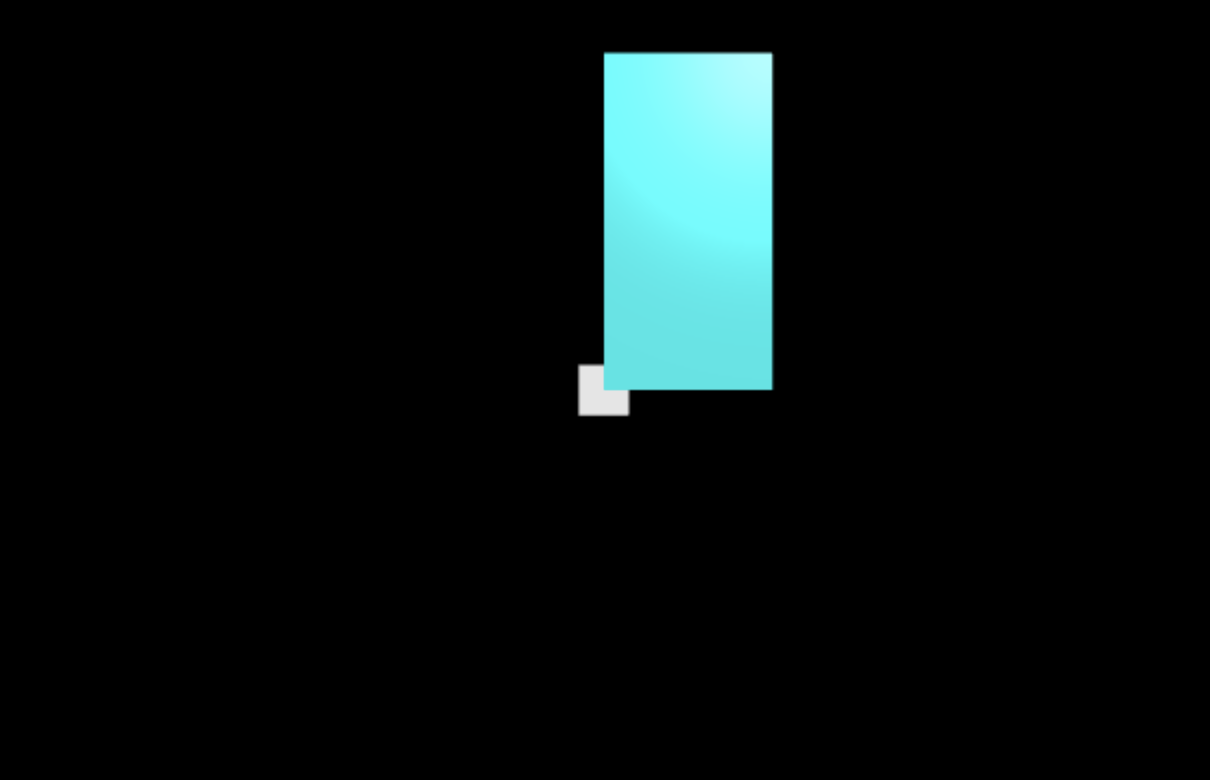
The following code adds a cyan colored box with dimensions <2, 4, 6> that is centered at <1, 2, 3> to the scene.

from vpython import *

box()
box(pos=vector(1, 2, 3), length=2, height=4, width=6, color=color.cyan)

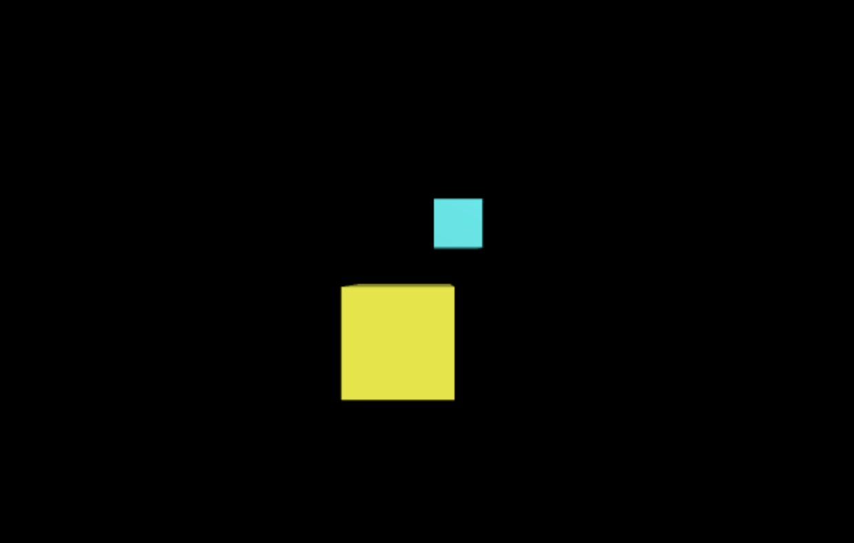
You can get the value of an attribute by using . notation. You can set custom attributes by using the same . notation. The following code uses the attributes of one box to create a new box.

from vpython import *

my_box = box(pos=vector(1, 2, 3), size=vector(2, 2, 2), color=color.cyan)
my_box.special_scaling_factor = 3.1415

your_box = box(pos=my_box.pos * -2, size=my_box.size * my_box.special_scaling_factor, color=color.yellow)

3) Making the Simulation

The following code draws a cube using the curve object. In the following sections, you will add on to this code to make the target simulation. Assume that the VPython library is imported in all of the coding questions (using from vpython import *).

from vpython import *

box_size = 5
v = box_size / 2
r = 0.05
c = color.black
box_bottom = curve(color=c, radius=r)
box_bottom.append([vector(-v,-v,-v), vector(-v,-v,v), vector(v,-v,v), vector(v,-v,-v), vector(-v,-v,-v)])
box_top = curve(color=c, radius=r)
box_top.append([vector(-v,v,-v), vector(-v,v,v), vector(v,v,v), vector(v,v,-v), vector(-v,v,-v)])
vert1 = curve(color=c, radius=r)
vert2 = curve(color=c, radius=r)
vert3 = curve(color=c, radius=r)
vert4 = curve(color=c, radius=r)
vert1.append([vector(-v,-v,-v), vector(-v,v,-v)])
vert2.append([vector(-v,-v,v), vector(-v,v,v)])
vert3.append([vector(v,-v,v), vector(v,v,v)])
vert4.append([vector(v,-v,-v), vector(v,v,-v)])

3.1) Adding a Marble

We'll start by adding a marble with some initial velocity inside of our cube.

Click Run Simulation to see the simulation that your code produces. Click Submit to verify that your code is correct.

Complete the function add_marble which adds a sphere with a radius of 0.5 anywhere inside the cube and returns it. Set a custom vel attribute to any non-zero vector to represent its initial velocity.

def add_marble(): marble = sphere(pos=vector(-2, -1, 2), radius=0.5, color=color.blue, make_trail=True, retain=100) marble.vel = vector(1, 2, 3) return marble

Run Simulation Save Submit View Answer Loading...

As staff, you are always allowed to submit. If you were a student, you would see the following:
You have infinitely many submissions remaining.

Let's take a second to talk about the output that you see when you click Run Simulation:

1. First, you'll see the actual simulation itself. You can interact with the scene using your mouse and keyboard.
   • Use shift+drag to pan the camera
   • Use control+drag to rotate the camera
   • Use option/alt+drag or scroll wheel to zoom
2. Next, you'll see some user input widgets, such as buttons, which can be used to interact with the simulation. Our simulation currently isn't moving so the Play/Pause button doesn't do anything yet.
3. After that, you'll see the console, which shows you the output of any print statements in your code.
4. Lastly, you'll see the code that was used to create the simulation. The "Make Sim UI" section is what makes the user interface for the simulation and everything below that is what actually draws and animates the simulation.

Now, let's look at our simulation logic.

marble = add_marble()

while True:
    rate(200)

Our simulation will use a while loop to continuously update our scene. The rate(200) controls the rate at which our scene is redrawn. It's a requirement for VPython to run the simulation correctly. Since we're not doing anything in our while loop, our scene stays the same.

3.2) Moving the Marble

Now that we have our marble in the scene, let's animate it!

Complete the function move_marble which updates the position of the marble according to its velocity over the given change in time dt. The function should return the marble.

def move_marble(marble, dt): marble.pos += marble.vel * dt return marble

Run Simulation Save Submit View Answer Loading...

As staff, you are always allowed to submit. If you were a student, you would see the following:
You have infinitely many submissions remaining.

Look at the new simulation code:

1. There is a new variable dt which represents the change in simulation time after one iteration of the while loop.
2. If the button is in "Play" mode, the marble moves according to the function you defined.

3.3) Colliding with the Walls

To prevent our marble from launching into the void, let's make it bounce off of the cube's walls. When the marble is out of bounds, its velocity should flip signs in the direction that it was out of bounds in.

Complete the function check_wall_collision which checks if a marble is out of bounds and updates the velocity of the marble accordingly. Remember that the box is centered around 0. Return the marble.

def check_wall_collision(marble, box_size): if abs(marble.pos.x) + marble.radius >= box_size / 2: marble.vel.x *= -1 if abs(marble.pos.y) + marble.radius >= box_size / 2: marble.vel.y *= -1 if abs(marble.pos.z) + marble.radius >= box_size / 2: marble.vel.z *= -1 return marble

Run Simulation Save Submit View Answer Loading...

As staff, you are always allowed to submit. If you were a student, you would see the following:
You have infinitely many submissions remaining.

3.4) Adding More Marbles

Now let's add more marbles to see them all bounce around in the cube! In the following question, feel free to use the vector.random() function if you would like to add some randomness to your simulation.

Complete the function add_other_marbles which adds n marbles inside of the cube, each with some initial velocity.

def add_other_marbles(box_size, n=4): other_marbles = [] for i in range(n): r = 0.5 bounds = box_size / 2 - r found_pos = False while not found_pos: pos = bounds * vector.random() collision = False for o_m in other_marbles: if mag(pos - o_m.pos) < r + o_m.radius: collision = True if not collision: found_pos = True s = sphere(pos=pos, radius=r) s.vel = 2 * vector.random() other_marbles.append(s) return other_marbles

Run Simulation Save Submit View Answer Loading...

As staff, you are always allowed to submit. If you were a student, you would see the following:
You have infinitely many submissions remaining.

Notice how we now have to iterate through our list of marbles at every iteration of our loop to update their position and check for wall collisions.

3.5) Marble Collisions

For our last trick, we will make the marbles collide with each other. Remember that for equal mass elastic collisions between spheres:

\vec{v}_2' = \vec{v}_2 - \left[ (\vec{v}_2 - \vec{v}_1) \cdot \hat{n} \right] \hat{n}

where \hat{n} = \frac{\vec{r}_1 - \vec{r}_2}{\left\lVert \vec{r}_1 - \vec{r}_2 \right\rVert} is the unit vector pointing from particle 2 to particle 1 (direction of collision), \vec{v}_1, \vec{v}_2 are the velocities before the collision, and \vec{v}_1', \vec{v}_2' are the velocities after the collision.

You may find the norm and dot functions useful in your calculations.

Complete the function check_marble_collision which checks if the given two marbles, m1 and m2, are colliding and, if so, updates their velocities according to the equation above. The function should return the two marbles.

def check_marble_collision(m1, m2): if mag(m1.pos - m2.pos) < m1.radius + m2.radius: n = norm(m1.pos - m2.pos) vel1_n = dot(m1.vel, n) vel2_n = dot(m2.vel, n) m1.vel = m1.vel - n*(vel1_n - vel2_n) m2.vel = m2.vel - n*(vel2_n - vel1_n) return [m1, m2]

Run Simulation Save Submit View Answer Loading...

As staff, you are always allowed to submit. If you were a student, you would see the following:
You have infinitely many submissions remaining.

Notice that in every iteration of our loop, we're now checking each marble pair to see if they're colliding. And with that, we've completed our simulation!

3.6) Graphing Data

VPython supports graphing data dynamically in real time. In order to graph data, we must first create a graph object. We use this object to style our graphing region (set the title, label our axes, etc.). Then, we can create a gcurve, gdots, or gvbars object using that graph object to make the plot itself.

In the following example, we use a gcurve object to plot the total momentum in the system over time. Since we are simulating perfectly elastic collisions, we should expect the total momentum to stay constant. Let's see how good our simulation actually is!

Run the following code to see plot it produces. Feel free to modify the code to plot other data.

g = graph(title='Total Momentum of the System', xtitle='Time (t)', ytitle='Momentum (kg * m/s)', ymin=0, ymax=100) plot = gcurve(graph=g) def update_plot(plot, all_marbles, t): total_momentum = 0 for m in all_marbles: total_momentum += 1 * mag(m.vel) plot.plot(t, total_momentum)

Run Simulation Save Submit View Answer Loading...

As staff, you are always allowed to submit. If you were a student, you would see the following:
You have infinitely many submissions remaining.

You can see that we added a t variable which tracks the total amount of simulation time that has passed. At every iteration of our loop, we update our plot using the update_plot function that we defined.